
As a Brazilian working for a foreign company, I'm always keeping an eye on the USD to BRL exchange rate to plan my finances for the month. In the first few months, I tried predicting the dollar rate on my payday using all sorts of methods: checking forecasts from financial institutions, looking into futures, using statistics, but none of them really worked. The value was always different from what I expected, sometimes higher, sometimes lower.
Because of that, I decided to write a post about time series forecasting. I wanted to dig deeper into why it's so hard to make accurate predictions and share some of the insights I’ve learned along the way.
3 rules to know if something can be predicted
Not everything can be forecasted, some assumptions need to be met.
Rule 1: We need to know and understand the factors that affect the indicator that we are trying to predict
Condition matched for Dollar Rate forecasting? ❌
The dollar rate is influenced by dozens of factors, and worse, many of them are unpredictable, or we simply don't know whether a change will push the rate up or down. Interest rates, inflation, political stability, commodity prices, global financial crises, wars, elections... the list goes on.
Even if you could model some of these factors (like Central Bank decisions or inflation rates), sudden geopolitical events or unexpected government actions can easily throw any forecast completely off track. We simply don't have access to all the variables at play.
Rule 2: There must be enough data available
Condition matched for Dollar Rate forecasting? ✅
This condition is certainly matched, since we have lots of historical data on the USD Rate against most of the currencies of the world. When we want to forecast something, it's important to have enough data, so we can correctly identify patterns, trends, and seasonality.
Rule 3: The forecast itself should not change the indicator value
Condition matched for Dollar Rate forecasting? ❌
For a forecast to be reliable, the act of making the prediction itself shouldn't influence the result. If everyone changes their behavior based on the forecast, the forecast stops being valid.
Imagine a big and respected financial institution, like Goldman Sachs, publishing a report saying:
"We expect the dollar to rise by 5% over the next month against the BRL."
Investors and companies don't want to miss the opportunity.
As soon as the report is published, there’s a rush to buy dollars, creating extra demand and making the dollar rise immediately.
Very likely, the price will reach — or even exceed — the predicted 5% rise before the month ends.
At that point, the original forecast becomes flawed: reality has already changed because of the forecast itself.
This is a classic effect described by the Efficient Market Hypothesis (EMH): In efficient markets, as soon as new information appears, prices adjust immediately. You can’t profit easily from forecasts, because once a prediction is public, the market incorporates it into the price.
Trying anyway
As we saw, only one of the three conditions was met, so we can assume that forecasting the Dollar Rate with precision is not possible, or at least extremely difficult.
But, since we are already here, let's try it anyway.
How to forecast time series data?
The first step in forecasting time series data is choosing a model.
The most popular models are:
- Moving Averages: smooth out short-term fluctuations to highlight longer-term trends or cycles.
- ARIMA (AutoRegressive Integrated Moving Average): combines autoregression, differencing (to make data stationary), and moving averages to predict future values.
- SARIMA (Seasonal ARIMA): an extension of ARIMA that also models seasonality patterns (like peaks that happen every year or month).
- Prophet: developed by Facebook, designed to handle time series with strong seasonal effects and holidays, with a more intuitive and flexible configuration.
- LSTM (Long Short-Term Memory networks): a type of recurrent neural network (RNN) capable of learning long-term dependencies, often used for complex time series where classical models struggle.
For this article, let's proceed with Prophet, since it's a very reliable, modern, and easy-to-use model. You can try with more sophisticated models if you want, such as custom LSTMs, NeuralProphet, and others.
Prophet
Prophet is an open-source library developed by Facebook designed to simplify the process of forecasting time series data. It has some assumptions:
- The data must have seasonality
- It assumes that the data has a trend, and that this trend can be shifted at different points in time
Currencies usually have a trend, their movement is not purely random, which is good for our model. However, the seasonality of currencies is not so simple, there are many factors involved. Despite this complexity, historical data reveals certain seasonal behaviors. For instance, the U.S. dollar typically experiences weakness in December, often attributed to year-end tax strategies by U.S. companies, and tends to reverse the performance in January, with a good performance.
Config
Let's begin by defining some parameters for our model, such as the date range for our prediction, the API KEY for the FRED API, which is where we will get data about the US interest rates, and some other info related to holidays and special dates.
import pandas as pd
import numpy as np
import matplotlib.pyplot as plt
import matplotlib.patches as mpatches
from datetime import datetime, timedelta
import requests
from prophet import Prophet
from fredapi import Fred
from prophet.make_holidays import make_holidays_df

# ====== CONFIG ======
FRED_API_KEY = os.getenv("FRED_API_KEY")

end_date = datetime.today()
start_date = end_date - timedelta(days=365 * 3)
start_str = start_date.strftime('%d/%m/%Y')
end_str = end_date.strftime('%d/%m/%Y')
start_iso = start_date.strftime('%Y-%m-%d')
end_iso = end_date.strftime('%Y-%m-%d')

url_usdbrl = f"https://api.bcb.gov.br/dados/serie/bcdata.sgs.1/dados?formato=json&dataInicial={start_str}&dataFinal={end_str}"
url_brazil_interest_rates = f"https://api.bcb.gov.br/dados/serie/bcdata.sgs.1178/dados?formato=json&dataInicial={start_str}&dataFinal={end_str}"

# COPOM is the committee that defines Brazil's interest rates
copom_meeting_dates = [
    # 2025
    "2025-06-18", "2025-05-07", "2025-03-19", "2025-01-29",
    # 2024
    "2024-12-11", "2024-11-06", "2024-09-18", "2024-07-31",
    "2024-06-19", "2024-05-08", "2024-03-20", "2024-01-31",
    # 2023
    "2023-12-13", "2023-11-01", "2023-09-20", "2023-08-02",
    "2023-06-21", "2023-05-03", "2023-03-22", "2023-02-01",
    # 2022
    "2022-12-07", "2022-10-26", "2022-09-21", "2022-08-03",
    "2022-06-15", "2022-05-04", "2022-03-16", "2022-02-02"
]
fed_meeting_dates = [
    # 2025
    "2025-12-17", "2025-11-05", "2025-09-17", "2025-07-30",
    "2025-06-18", "2025-05-07", "2025-03-19", "2025-01-29",
    # 2024
    "2024-12-11", "2024-11-06", "2024-09-18", "2024-07-31",
    "2024-06-12", "2024-05-01", "2024-03-20", "2024-01-31",
    # 2023
    "2023-12-13", "2023-11-01", "2023-09-20", "2023-07-26",
    "2023-06-14", "2023-05-03", "2023-03-22", "2023-02-01",
    # 2022
    "2022-12-14", "2022-11-02", "2022-09-21", "2022-07-27",
    "2022-06-15", "2022-05-04", "2022-03-16", "2022-01-26"
]
us_holidays = make_holidays_df(
    year_list=[2019 + i for i in range(10)], country='US'
)
br_holidays = make_holidays_df(
    year_list=[2019 + i for i in range(10)], country='BR'
)
Fetching the historical data for USD-BRL
response = requests.get(url_usdbrl)
data_usdbrl = response.json()

df_usdbrl = pd.DataFrame(data_usdbrl)
df_usdbrl['ds'] = pd.to_datetime(df_usdbrl['data'], format='%d/%m/%Y')
df_usdbrl['y'] = df_usdbrl['valor'].astype(float)
df_usdbrl = df_usdbrl[['ds', 'y']]
Adding regressors to enhance our model's performance
A regressor can be any variable in a regression model that is used to predict a response variable. Prophet allows us to add multiple regressors, so we will have 2:
- Interest Rates
- Central Bank Meeting Dates
*We also have the holidays, but they are not considered external regressors, since they are "part of the equation".
Interest Rates
# ====== GETTING INTEREST RATES FROM BRAZIL ======
response = requests.get(url_brazil_interest_rates)
data_selic = response.json()

df_selic = pd.DataFrame(data_selic)
df_selic['ds'] = pd.to_datetime(df_selic['data'], format='%d/%m/%Y')
df_selic['selic'] = df_selic['valor'].astype(float)
df_selic = df_selic[['ds', 'selic']]

# Fill missing dates if needed
today = pd.to_datetime(datetime.today().date())
if today not in df_selic['ds'].values:
    last_selic = df_selic.sort_values('ds')['selic'].iloc[-1]
    new_row = pd.DataFrame({'ds': [today], 'selic': [last_selic]})
    df_selic = pd.concat([df_selic, new_row], ignore_index=True)
    df_selic = df_selic.sort_values('ds').reset_index(drop=True)

# ====== GETTING INTEREST RATES FROM US ======
fred = Fred(api_key=FRED_API_KEY)
fedfunds = fred.get_series('FEDFUNDS', observation_start=start_iso, observation_end=end_iso)

df_fedfunds = fedfunds.reset_index()
df_fedfunds.columns = ['ds', 'fedfunds']
df_fedfunds['ds'] = pd.to_datetime(df_fedfunds['ds'])
df_fedfunds['fedfunds'] = df_fedfunds['fedfunds'].astype(float)
full_dates = pd.DataFrame({'ds': pd.date_range(start=df_fedfunds['ds'].min(), end=df_selic['ds'].max())})
df_fedfunds = full_dates.merge(df_fedfunds, on='ds', how='left')
df_fedfunds['fedfunds'] = df_fedfunds['fedfunds'].ffill()

# ====== MERGING IT ALL ======
df = df_usdbrl.merge(df_selic, on='ds', how='left')
df = df.merge(df_fedfunds, on='ds', how='left')
Central Bank Meeting Dates
# ====== CREATE DATAFRAME WITH MEETINGS DATES ======
copom_df = pd.DataFrame(copom_meeting_dates, columns=["ds"])
copom_df["ds"] = pd.to_datetime(copom_df["ds"])
fed_df = pd.DataFrame(fed_meeting_dates, columns=["ds"])
fed_df['ds'] = pd.to_datetime(fed_df['ds'])

all_meetings_df = pd.concat([copom_df, fed_df]).drop_duplicates().sort_values("ds").reset_index(drop=True)

# ====== CATEGORIZE IF IT'S NEAR A CENTRAL BANK MEETING ======
def is_near_central_bank_meeting(date, days_before=5, days_after=1):
    date = pd.to_datetime(date)
    for meeting_date in all_meetings_df['ds']:
        if -days_before <= (date - meeting_date).days <= days_after:
            return 1
    return 0

df['near_cb_meeting'] = df['ds'].apply(is_near_central_bank_meeting)
Setting up the Holidays
# Add a new column to distinguish between the two countries
us_holidays['country'] = 'US'
br_holidays['country'] = 'BR'

# Concatenate the two DataFrames into a single one
combined_holidays = pd.concat([us_holidays, br_holidays], ignore_index=True)
Instantiate the model and plug the regressors
Now we enter our final step: create the model, plug the regressors we have previously created, and then run it to forecast the dollar rate for the next 45 days.
model_prophet = Prophet(
    changepoint_range=0.9,
    changepoint_prior_scale=0.1,
    yearly_seasonality=True,
    weekly_seasonality=True,
    daily_seasonality=False,
    holidays=combined_holidays
)
model_prophet.add_regressor('near_cb_meeting')
model_prophet.add_regressor('selic')
model_prophet.add_regressor('fedfunds')
model_prophet.fit(df)

# ====== FORECAST ======
future = model_prophet.make_future_dataframe(periods=45)
future['near_cb_meeting'] = future['ds'].apply(is_near_central_bank_meeting)

last_selic = df['selic'].ffill().iloc[-1]
last_fedfunds = df['fedfunds'].ffill().iloc[-1]
future = future.merge(df[['ds', 'selic', 'fedfunds']], on='ds', how='left')
future['selic'].fillna(last_selic, inplace=True)
future['fedfunds'].fillna(last_fedfunds, inplace=True)

forecast_prophet = model_prophet.predict(future)
Interpreting the results
To better interpret the results, it is essential that we visualize them, so let's plot some charts:
Forecast of the USD/BRL Exchange Rate Considering Central Bank Meetings
The chart above shows the forecast of the USD/BRL exchange rate using the Prophet model. The black dots represent historical exchange rate values. The blue line in the middle is the main prediction made by the model for each day, it’s not a trend, but the central estimate of where the exchange rate is expected to be.
The shaded blue area around the line shows the uncertainty in the forecast. It gives us an idea of how much the exchange rate could go up or down at this point in time, based on the model's confidence (80% by default). The further into the future, the wider this area gets, reflecting more uncertainty.
The dashed orange vertical lines mark the dates of Central Bank meetings in Brazil and the US, which can have a strong impact on the exchange rate, especially if there are changes in interest rates or economic outlook.

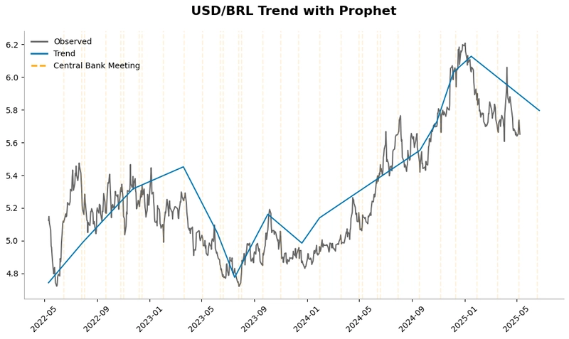
USD/BRL Trend
The chart above shows the underlying trend of the USD/BRL exchange rate over time, extracted using Prophet’s trend component. The black line represents the observed exchange rate, while the blue line shows the long-term movement of the exchange rate, smoothing out short-term fluctuations.
We can clearly see that forecasting the trend gives us much more accurate results than trying to predict the exact dollar rate at a specific point in time. The trend, if well modeled, won't be affected by short-term fluctuations and outliers. By visualizing the trend, it becomes easier to identify structural movements over time.
Validating the Results
To assess the accuracy of the USD/BRL forecast model, we performed cross-validation using Prophet. The training window was set to two years, and new forecasts were generated every 15 days for a 45-day horizon.
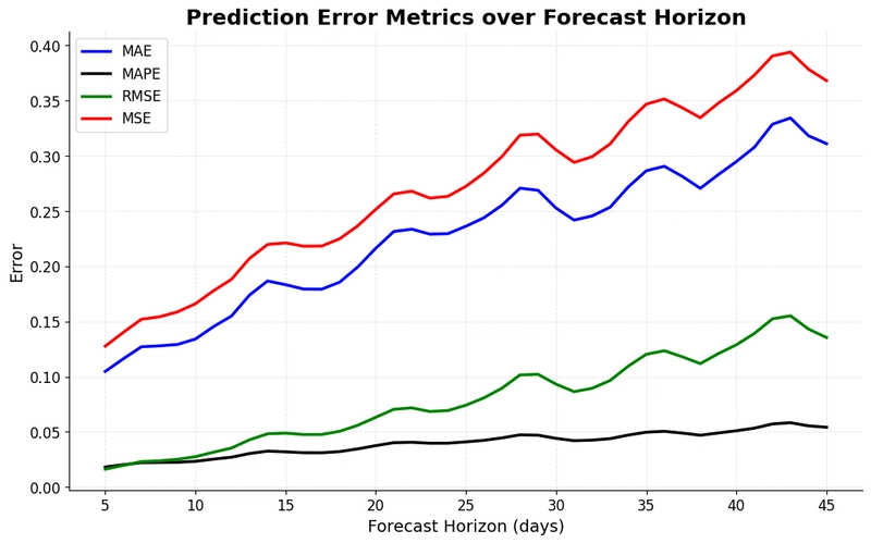
The chart above presents the error metrics across the forecast horizon:
- MAE (Mean Absolute Error) – shown in blue – quantifies the average absolute difference between predicted and actual values. It increases steadily with the horizon, reflecting the growing difficulty of long-term forecasting.
- MAPE (Mean Absolute Percentage Error) – shown in black – it is like MAE, but in percentage, showing a percentage of how much the values differ. We can see that it is under 5% most of the time, which is excellent.
- RMSE (Root Mean Squared Error) – shown in green – gives more weight to larger errors. It remains the second lowest among the four metrics, but still shows a clear upward trend.
- MSE (Mean Squared Error) – shown in red – grows consistently and sharply across the forecast window, indicating increasing squared deviations from actual values.
This diagnostic confirms a common behavior in time series forecasting: prediction errors tend to increase as we forecast further into the future. The consistent upward trajectory across all metrics reinforces the need to interpret longer-horizon forecasts with more caution.
Limitations of forecast accuracy in the face of unpredictable events
Even though the error metrics (MAE, MAPE, RMSE, MSE) for short-term horizons like 5, 10, or 15 days ahead are relatively low, indicating that the model performs well under normal conditions, it is essential to recognize the inherent unpredictability of exchange rate dynamics, particularly for the USD/BRL pair.
Exchange rates are highly sensitive to macroeconomic shocks and geopolitical events, many of which are impossible to anticipate using historical patterns alone. For example:
- A foreign government could announce a major monetary policy shift (e.g., unexpected interest rate cuts, capital controls, or intervention in currency markets) over a weekend, while markets are closed. When trading resumes, the exchange rate can experience a sudden gap that no model can foresee.
- Similarly, unforeseen global events, such as military conflicts, health crises, or abrupt changes in commodity prices, can trigger volatility spikes that exceed the bounds of even the most accurate statistical forecasts.
These scenarios expose that we cannot capture "black swan" events or model the reactions of market participants to breaking news.
How to improve the model?
The model we built in this article isn't perfect, and surely it can be improved, but how? Here are some suggestions for you to try by yourself:
- Gather news and perform sentiment analysis on social media to understand how the market is reacting
- Track commodities prices as a regressor
- Try to replace Prophet with NeuralProphet or a custom LSTM
- Add other economic indicators like inflation, or unemployment
- Combine different models and compare their performance
There’s a lot to explore here, and testing different approaches is part of the fun.
You can check the full code here: https://github.com/josethz00/dollar-forecast


Top comments (0)